| Content Type |
Application |
Author |
Price |
| Macro |
Microsoft Excel |
OfficeHelp |
Free |
ExMiniTools - Utilities Toolbar for Microsoft® Excel® - Version 2.00
Tested on Microsoft Excel Versions: 2000 (9.0), XP (10.0), 2003 (11.0), 2007 (12.0), 2010 (14.0), 2013, 2016 - should work on any version from Office 97 |
|
Additional Functions & 1 Click Buttons for Excel® with AUTOMATIC SORTING (data changed? just recalculate to sort), EXACT COPY/PASTE (no formula changes), COMPARE FORMULAS in 2 ranges, COUNT UNIQUE values in ranges, RANK numbers in a range (is it the 1st or 4th?), RESTORE ADDIN FUNCTIONS (automatically remove file path from functions), apply ALTERNATE BACKGROUNDS (Row/Column) for easier table reading, automatically REMOVE #ERRORS and 1 Click access to 9 common features. |
|
MANUAL - Toolbar Buttons & Worksheet Functions Reference

How-To
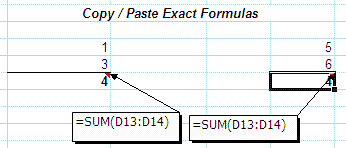
Copy/Paste Exact Formulas
Copy/Paste a range of cells without Excel adjusting the cell references in formulas within it. Follow these steps:
1) Select a contiguous range of cells and click on the Memorizes Selected Cells ( ) Toolbar button. ) Toolbar button.
- Do not use Excel regular COPY. You need to use this specific toolbar button.
2) Select the Top Left cell on the intended Paste range. Click on the Paste Exact Formulas ( ) Toolbar button to paste the exact formulas of the original range. ) Toolbar button to paste the exact formulas of the original range.
3) The formulas on the new "pasted" range are EXACTLY as the original one. No adjustments will be done the the formulas and cell references.
Create an Auto-Sorted Table
This innovative feature is intended to provide auto-sorted tables in Excel,
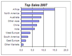
really useful to create rankings and Rank charts:
Create Rankings (Top Sellers)
 |
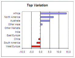
Actual to Budget variations
 |
While you can manually sort ranges in Excel, this is a
manual and tiresome process, especially if it has to be done
regularly (daily, weekly or monthly reports) and on several
tables. It would be much easier if you could just update the
data and recalculate to reorder the table!
Instead of sorting the original table, we create a new one (linked to the original) that will always sort itself when recalculated:
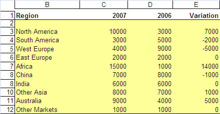
(Row and Column headings shown):
Original Data Table
 |
Sorted Table
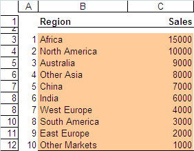 |
On the sorted table, we need a column to indicate each row order number (A) and a cell to indicate the sort order
(TRUE = Ascending, FALSE = Descending). For each cell, enter a call to
the TopN() function:
=TopN($C$14:$C$23; A34; "C";$H$8)
The exact syntax of this function is:
= TopN (nRange, TopNVal, ReturnCol, SortType)
- nRange: Range of cells for the Ranking. Can have only ONE column.
- TopNVal: Index number in Ranking to be returned (1 for first, 2 for second,…)
- ReturnCol: Column number were to fetch the return value
-
SortType: Sort Order for the cell values:
- TRUE: ASCENDING
- FALSE: Descending
This function will return the Nth member of the original table, sorted by
the indicated nRange. So, to retrieve the 3rd largest region in
2007, we need to define the function as:
- nRange: $C$3:$C$$12 (values for 2007)
- TopNVal: 3 (as a number, for 3rd) or a reference to the
order column on the sorted table (A5)
- ReturnCol: "B" to return the region name or "C" to return
the region value.
-
SortType: TRUE (ascending)
So to create the Sorted table we use the the same function (as above) and
only change the ReturnCol parameter in order to retrieve the
region labels and value.
It is also possible to return secondary values based on another column sort
order
(like returning variances to Budget and Last Year based on the “variance to Budget” sort order – the variances to Last Year will not be retrieved sorted by itself by sorted by the
“variance to Budget” values). Creating the new column is as easy as copying one of the existing ones (either labels or values) and changing the
ReturnCol parameter (the column to be
returned).
In the example above, a 3rd column could be added to the Sorted Table to
indicate the variation to 2006, keeping it sorted by 2007 values. The only
change would be, again the ReturnCol parameter, that in this case
would have to be set to "E", retrieving the Variation column of the Original
Data Table. The final Sorted Table would use these formulas on the first row
(3):
- Column "B" - Label (sorted by 2007 values): =TopN($C$3:$C$$12; A5; "B"
TRUE)
- Column "C" - 2007 Values (sort column): =TopN($C$3:$C$$12; A5; "C"
TRUE)
- Column "D" - Variation to 2006 (sorted by 2007 values): =TopN($C$3:$C$$12; A5; "E"
TRUE)
These formulas (for the first row), could then be dragged down until the 10
rows were filled.
Compare Formulas in 2 Ranges
Compare the formulas within 2 cell ranges. Follow these steps:
1) Select a contiguous range of cells and click on the Memorizes Selected Cells ( ) Toolbar button. ) Toolbar button.
- Do not use Excel regular COPY. You need to use this specific toolbar button.
2) Select the Top Left cell on the intended comparison range. Click on the Formula Comparison ( ) Toolbar button. ) Toolbar button.
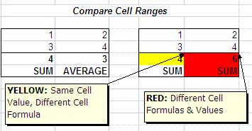
3) Each cell on the comparison range will be compared with its similar cell on the original range. Cells will be painted according to the comparison results:
- YELLOW: Same value as reference cell, but formula is different
- RED: Different value and formula compared to reference
- NONE: No difference to reference (same value and formula)
Apply Backgrounds to Ranges / Tables
Apply alternate backgrounds (Row/Column) in a single click - Much easier to read, specially in print. Just Select & Apply
1) Format cell A1 (on the active worksheet) with the desired background color. This cell will be the reference
2) Apply the desired background pattern. Cell A1 background format will be applied to the selected range:
- Alternate Rows (
 ) - Applies a background color to
alternate rows of the current selection. ) - Applies a background color to
alternate rows of the current selection.
- Alternate Columns (
 ) - Applies a background color to
alternate columns of the current selection. ) - Applies a background color to
alternate columns of the current selection.
- Chess Pattern (
 ) - Applies a background color to
alternate cells of the current selection, creating a “Chess Pattern”. ) - Applies a background color to
alternate cells of the current selection, creating a “Chess Pattern”.
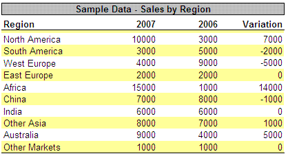
3) The selected range will be formatted with the desired pattern (example: Alternate Rows pattern):
Automatically repair broken function links from AddIns
Excel treats external functions residing in AddIns as
links. Therefore, when the file using them is saved, it will add the full
path the AddIn to the function call in the cells:
Entered in File: =topn($C$14:$C$23; A32; "C";$H$8)
After Saving: =C:\Program Files\AddIn\ThisAddIn.xla!topn($C$14:$C$23;
A32; "C";$H$8)
This is a real problem if the file is later opened in a different computer
where the AddIn resides in a different disk location, as Excel will consider
the link broken and will not calculate the AddIn functions until the disk
path is removed. This can be very frustrating as some files may have
thousands of function calls needing cleaning. This is a common scenario for
corporate users using Excel Addins to retrieve data from their corporate
databases and Business Intelligence or Financial applications.
To use this feature, just open the file needing the restore and click the
 button. The Toolbar will check ALL cells with functions on the active
workbook and restore the AddIn function calls in all cells needing it. There
is no need to select ranges or sheets, it will apply to the whole active
workbook. Once done, just save the file to disk.
Remove all #Errors from a Range
This feature is intended to clean tables of error cells (like #Div/0)
before copying to Word or printing. Cells with errors (shown starting with a
# in Excel) will be ERASED permanently, because this errors may cause other
cells (like SUMs) to also show errors instead of calculating the remaining
values. It is therefore advisable to use it on a copy of the original sheet.

To use it select an range of cells with the mouse and click on the  button. The toolbar will check each cell in the selected range and, if it
contains an Excel calculation error, it will be erased. The final range will
only have values and empty cells, resulting in a “clean” table for printing
purposes.
1 Click access to Excel commands
SAVE TIME with direct, 1 click access to the "hidden" Excel commands. This buttons will invoke the regular Excel commands performing the same functions.
-
Calculate
- Calculate Active Sheet (
 ) )
- Calculate Selected Range (
 ) )
- Calculate Active Workbook only (F9 will calculate all open workbooks) (
 ) )
- Manual / Automatic Calculation mode Toggle (
 ) )
|
-
Paste
- Paste Values (
 ) )
- Paste Formulas (
 ) )
- Paste Formats (
 ) )
|
|
|
|
Install an Excel AddIn (not necessary for the DEMO, only for the full
product)
An Excel AddIn is an extension to Excel and, once installed, will load every
time Excel is loaded, becoming “part” of Excel until it is deliberately
uninstalled. Learn how to install and manage them on all versions of Excel
from 97 to 2007.
- The free DEMO for this product is intended for testing
purposes only and is not an AddIn but a plain Excel file. Just
open it with macros enabled and the new Toolbar withh be added to Excel
for immediate use.
- The full product is an Excel AddIn and can be
installed to be loaded with Excel every time it starts.
Click here for an
illustrated article on How to Install Excel AddIns.
TOOLBAR BUTTONS
|
WORKSHEET FUNCTIONS
|
Calculation Group
|
 |
Calculates Active Sheet (Only)
Calculates the active sheet. Useful to force its calculation when in MANUAL calculation mode. Similar to
the "Calc Sheet" button in the Tools / Options menu.
|
 |
Calculates Selected Cells (Only)
Calculates the current selection. Useful to force its calculation when in MANUAL calculation mode. Not
available on Excel(R) menus.
|
 |
Calculates All Sheets from Current Workbook
Calculates the current workbook by looping all worksheets twice.
Not available on Excel(R) menus.
|
 |
Toggles Calculation between MANUAL and AUTOMATIC
When clicked, it will change the calculation mode.
If in MANUAL, it will change to AUTOMATIC.
If in AUTOMATIC, it will change to MANUAL
|
Ranges Group
|
 |
Memorizes Selected Cells
Memorizes the formulas (not values) of all cells on the current selection. For use with the other buttons within this group.
|
 |
Formula Comparison
Compares formulas between the memorized area (button above) and the area starting on the current selected cell. Cells with differences are painted red (background color).
|
 |
Paste Exact Formulas
Works like Paste Formulas but makes NO adjustments to the copied formulas. Pastes the memorized cells to the Range starting with the current selected cell.
WARNING: The original cells have to be MEMORIZED, not COPIED with Copy.
|
Paste Group
|
 |
Paste Values
Shortcut to the Paste Values option on the Paste Special pop-up. Pastes only the Values of the current Copy source (need a previous Copy).
|
 |
Paste Formulas
Shortcut to the Paste Formulas option on the Paste Special pop-up. Pastes only the Formulas of the current Copy source (need a previous Copy). Relative formulas will be adjusted (cell
references change) as usually in Excel.
For an Exact Formula paste (not available in standard Excel), see Paste Exact Formulas above.
|
 |
Paste Formats
Shortcut to the Paste Formats option on the Paste Special pop-up. Pastes only the Formats of the current Copy source (need a previous Copy), applying the source formats to the target
cells without changing their formulas.
|
Grid Group
|
 |
Alternate Rows
Applies a background color to alternate rows of the current selection. Useful to make easier reading of large tables, especially on prints. Uses cell A1 background as reference
(copies its background).
|
 |
Alternate Columns
Applies a background color to alternate columns of the current selection. Useful to make easier reading of large tables, especially on prints. Uses cell A1 background as reference
(copies its background).
|
 |
Chess Pattern
Applies a background color to alternate cells of the current selection, creating a “Chess Pattern”. Useful to make easier reading of large tables, especially on prints.
Uses cell A1 background as reference (copies its background).
|
Other Buttons
|
 |
Remove disk path to restore AddIn formulas
Checks ALL cells with formulas in ALL sheets of the current workbook and removes disk path links to external formulas (like the ones in this Toolbar). Restores formulas with external
AddIn functions allowing them to work again. Excel adds a full disk path to AddIn files when you use formulas in external AddIns, like the one in this Toolbar but also many others,
including Microsoft own and the ones from most Enterprise software vendors. This can be highly annoying when someone else opens the file and the AddIn is located in a different
location, as the functions WILL NOT WORK.
|
 |
Remove # Errors for Illustration Purposes
Erases formulas with # errors within cells on the current SELECTION. This is definitive so it should be used with care. Very useful when you need to copy large tables for illustration
purposes on Word or PowerPoint.
|
 |
About
Open a pop-up windows with additional information about this product. Include links to several related pages on OfficeHelp.Biz website, including Help/Manual, Commercial information
and Upgrade/Purchase pages.
|
|
|
Automatic Sorting & Ranking
IndexInRankingNum (nRange, SearchVal, SortType)
Returns the Index of a given value in a sorted table (Ranking Index)
Sort is numeric (9 comes before 10) and therefore both the range and Search values must be numeric (text is not supported).
- nRange: Range of cells for the Ranking. Each cell will be ranked by value
- SearchVal: Number whose order (index) in the Ranking is being searched
-
SortType (TRUE/FALSE): Sort Order for the Ranking:
- TRUE: Ascending
- FALSE: Descending
IndexInRankingTxt (nRange, SearchVal, SortType)
As above but for text values. Orders are performed as text, not numeric values, so 10 comes before 9 because it starts with a 1.
TopN (nRange, TopNVal, ReturnCol, SortType)
Returns the Nth value of a ranking (ordered) Range. The Range has to be single column. Can return any column (even outside of the Range), like Label or Value.
- nRange: Range of cells for the Ranking. Can have only ONE column.
- TopNVal: Index number in Ranking (1 for first, 2 for second,…)
- ReturnCol: Column number were to fetch the return value
-
SortType: Sort Order for the cell values:
- TRUE: ASCENDING
- FALSE: Descending
CountUnique (nRange)
Returns the number of different unique values in a given range. Like Excel standard Count() function but EXCLUDING repeats.
- nRange: Range of cells for the Ranking. Each cell will be ranked by value
Click here for a FREE DEMO for the Sheet Functions
Date Functions
GetEasterDate (Year)
Returns the date of the Easter Day for the given year.
Ex: GetEasterDate(2001) will return 15 of April 2001
AddWorkingDays (StartDate, NDays, Holidays)
Adds Working Days to a Start Date, discounting Weekends and Holidays into consideration. Weekend tracking is automatic but Holidays have to be supplied as a comma separated list of
dates.
Ex: AddWorkingDays(1/1/2006, 15, “'1/1/2006, 1/4/2006”) will return 1/20/2006
Click here for a FREE DEMO for the Sheet Functions
|
| |
| Download FREE Demo |
|
| EXCEL ONLY - No setup required. Just add to Excel AddIns and run! |
|
ExMiniTools - Utilities Toolbar for Microsoft® Excel® - Version 2.00
Tested on Microsoft Excel Versions: 2000 (9.0), XP (10.0), 2003 (11.0), 2007 (12.0), 2010 (14.0), 2013, 2016 - should work on any version from Office 97 |
|
|

